Homogeneous polynomial
In mathematics, a homogeneous polynomial is a polynomial whose monomials with nonzero coefficients all have the same total degree.[1] For example, 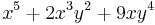 is a homogeneous polynomial of degree 5, in two variables; the sum of the exponents in each term is always 5. The polynomial
 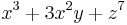 is not homogeneous, because the sum of exponents does not match from term to term. An algebraic form, or simply form, is another name for a homogeneous polynomial. The theory of algebraic forms is very extensive, and has numerous applications all over mathematics and theoretical physics.
A homogeneous polynomial of degree 0 is simply a scalar, while a homogeneous polynomial of degree 1 is a linear functional, also known as a covector. A homogeneous polynomial of degree 2 is a quadratic form, and, away from 2 (in a ring where 2 is invertible), may be identified with a symmetric 2-tensor, simply represented as a symmetric matrix, though at 2 there is a difference between quadratic forms and symmetric forms, notably for integral quadratic forms. Higher degree homogeneous forms may likewise be identified with symmetric k-tensors so long as  is invertible.
Contents |
Symmetric tensors
Homogeneous polynomials are closely related to symmetric tensors, and are often confused with them. In general they are different concepts, but in many important cases they can be identified as identical: there is a natural map from symmetric tensors to homogeneous polynomials, and from homogeneous polynomials to symmetric polynomials, and these can often be chosen to be isomorphisms, inverse to each other; see quadratic form: symmetric forms for discussion for quadratic forms.
Most significantly, over the real or complex numbers symmetric tensors are identical to homogeneous polynomials, but over the integers they are distinct concepts, as discussed at integral quadratic form.
In general, over a field of characteristic zero symmetric tensors and homogeneous polynomials are naturally identified, and more generally if  is invertible,[note 1] then symmetric d-tensors can be identified with homogeneous polynomials of degree d.
The distinction is that symmetric d-tensors  are a subspace of the set of all d-tensors
  the invariants under the symmetric group
  –
–  while homogeneous polynomials
  are a quotient space of the d-tensors, the coinvariants under the symmetric group
  this can be done for all grades of tensors, yielding:
There is thus a natural inclusion of symmetric tensors in tensors, then quotienting to polynomials, yielding  there is further a symmetrization map from polynomials to symmetric tensors,
  but in general neither of these maps need be onto or one-to-one. For example, not every integral quadratic form arises from a symmetric 2-form:
  does not, but
  does.
does.
Details
Let X and Y be vector spaces; then homogeneous polynomials in X of degree d, taking values in Y, and symmetric d-tensors from X to Y are defined and related as follows.
Let T be a multi-linear map (tensor), which need not be symmetric:

Define the diagonal morphism  as
as
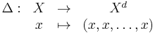
The homogeneous polynomial  of degree d associated with T is simply
  , so that

Written this way, it is clear that a homogeneous polynomial is a homogeneous function of degree d. That is, for a scalar a, one has
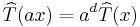
which follows immediately from the multi-linearity of the tensor.
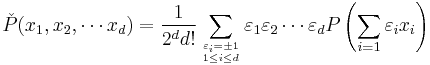
Conversely, given a homogeneous polynomial  , one may construct the corresponding symmetric tensor
  by means of the polarization formula or "symmetrization map":
Let  denote the space of symmetric tensors of rank d, and let
  denote the space of homogeneous polynomials of degree d. If the vector spaces X and Y are over the reals or the complex numbers, more generally, over a field of characteristic zero, most generally if
  is invertible, then these two spaces are isomorphic, with the mappings given by hat and check:

and

Algebraic forms in general
Algebraic form, or simply form, is another term for homogeneous polynomial. These then generalise from quadratic forms to degrees 3 and more, and have in the past also been known as quantics. To specify a type of form, one has to give its degree of a form, and number of variables n. A form is over some given field K, if it maps from Kn to K, where n is the number of variables of the form.
A form over some field K in n variables represents 0 if there exists an element
- (x1,...,xn)
in Kn such that at least one of the
- xi (i=1,...,n)
is not equal to zero.
Basic properties
The number of different homogeneous monomials of degree M in N variables is 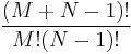
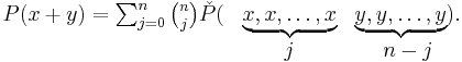
The Taylor series for a homogeneous polynomial P expanded at point x may be written as
Another useful identity is

Homogenization
A non-homogeneous polynomial  can be homogenized by introducing an additional variable
  and defining[2]
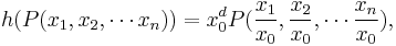
where  is the degree of . For example,
  .
.
A homogenized polynomial can be dehomogenized by setting the additional variable  .
.
History
Algebraic forms played an important role in nineteenth century mathematics.
The two obvious areas where these would be applied were projective geometry, and number theory (then less in fashion). The geometric use was connected with invariant theory. There is a general linear group acting on any given space of quantics, and this group action is potentially a fruitful way to classify certain algebraic varieties (for example cubic hypersurfaces in a given number of variables).
In more modern language the spaces of quantics are identified with the symmetric tensors of a given degree constructed from the tensor powers of a vector space V of dimension m. (This is straightforward provided we work over a field of characteristic zero). That is, we take the n-fold tensor product of V with itself and take the subspace invariant under the symmetric group as it permutes factors. This definition specifies how GL(V) will act.
It would be a possible direct method in algebraic geometry, to study the orbits of this action. More precisely the orbits for the action on the projective space formed from the vector space of symmetric tensors. The construction of invariants would be the theory of the co-ordinate ring of the 'space' of orbits, assuming that 'space' exists. No direct answer to that was given, until the geometric invariant theory of David Mumford; so the invariants of quantics were studied directly. Heroic calculations were performed, in an era leading up to the work of David Hilbert on the qualitative theory.
For algebraic forms with integer coefficients, generalisations of the classical results on quadratic forms to forms of higher degree motivated much investigation.
See also
- diagonal form
- graded algebra
- Homogeneous function
- multilinear form
- multilinear map
- polarization of an algebraic form
- Schur polynomial
- Symbol of a differential operator
Notes
Note notes
- ^ Properly, the polarization identity requires to be invertible, but repeated factors of 2 can be eliminated, 2 is already included in for
 and for
  these are both simply linear functionals.